Part 2 Using msm for a basic model
Model the progression through time of joint damage in psoriatic arthritis
Estimate, e.g.
probability that someone with no damaged joints (state 1) will have 10 or more damaged joints (state 4) 5 years from now.
Total time expected to spend over the next 10 years with 10 or more damaged joints.
No covariates for the moment - these will be introduced in Chapter 4.

Figure 2.1: Psoriatic arthritis
2.1 Basic requirements for a msm model
At minimum, need to specify
The dataset, and which columns indicate the state, time (and patient)
States should be numbers, 1, 2, 3, etc.
Time should be increasing within each patient (but first observation doesn’t have to be at time 0)
Patients should be grouped together in the data
The transition structure of the model
2.2 Summarising the data
Example psor dataset in the package
library(msm)
head(psor, 5)
## ptnum months state hieffusn ollwsdrt
## 1 1 6.46 1 0 1
## 2 1 17.08 1 0 1
## 3 2 26.32 1 0 0
## 4 2 29.48 3 0 0
## 5 2 30.58 4 0 0ptnum: subject / patient IDmonths: months of follow upstate: state of joint damage
Other columns are covariates, to be discussed later.
Each row represents a different time when the state was observed (not a time of transition!). Recall that the times of transition are not known in intermittently observed data.
A simple summary of the data is a count of the number of transitions over visit intervals, i.e. the number of people observed in one state at one visit, and each other state at the next visit.
statetable.msm(state, ptnum, data=psor)## to
## from 1 2 3 4
## 1 183 56 16 8
## 2 0 100 35 18
## 3 0 0 48 37For example, 16 people were in state 1 (0-1 damaged joints) at one visit followed by state 3 (5-9 damaged joints) at the next visit.
We also want some idea of the time scale, so we summarise the time variable.
summary(psor$months)## Min. 1st Qu. Median Mean 3rd Qu. Max.
## 0.1 3.5 7.3 10.0 13.1 57.1The inter-visit times, and number of observations per patient, may also be interesting to summarise.
2.3 Specifying the transition structure
We now define in R which transitions are allowed in continuous time
Define a matrix with \(r\), \(s\) entry
0 where the \(r\),\(s\) transition is disallowed
1 where the transition is allowed (actually this can be any non-zero positive number)
In this example we allow transitions from state 1 to state 2, from 2 to 3, and from 3 to 4.
Q <- rbind(c(0, 1, 0, 0),
           c(0, 0, 1, 0),
           c(0, 0, 0, 1),
           c(0, 0, 0, 0))
The diagonal entries of this matrix do not matter.
2.4 Transition structure is for the continuous time process
Note that when we used statetable.msm to summarise the transitions over visit intervals we counted 16 people in state 3 at the next visit after being observed in state 1.
So why do we not allow a State 1 to State 3 transition?
Because these 1-3 transitions happened over a time interval, not in continuous time
These 16 people must have gone through state 2 (unobserved) in between their visits
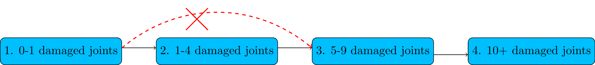
Multi-state models are commonly used in situations like this, for ordered states of disease severity, e.g. with states derived by discretising a continuous variable. Transitions should then only be allowed between adjacent states in continuous time.
The transition structure Q should not be chosen based on which elements of the statetable.msm output are non-zero!
Instead, it should be based on scientific judgement about what happens in continuous time.
2.5 Maximum likelihood estimation
Now we invoke the msm function to fit the multi-state model to the data: estimating the transition
intensities.
This uses optim to find the minimum of the minus log likelihood. It has to start this search from plausible initial values for the parameters. Two ways to do this:
Easiest way that usually works: tell
msmto auto-generate initial values with the argumentgen.inits=TRUE.psor.msm <- msm(state ~ months, subject = ptnum, data = psor, qmatrix = Q, gen.inits=TRUE)Alternatively: supply initial values yourself in the
qmatrix, instead of 1s, in the positions corresponding to the transitions.If you do this for different initial values, and it converges to the same answer, that gives reassurance that the answer is the true maximum likelihood estimate.
Q <- rbind(c(0, 0.1, 0, 0),
           c(0, 0, 0.1, 0),
           c(0, 0, 0, 0.1),
           c(0, 0, 0, 0))
psor.msm <- msm(state ~ months,
                subject = ptnum,
                data = psor,
                qmatrix = Q,
                gen.inits=TRUE)
But if we supply our own initial values, where would we get them from?
2.6 Intuition for what transition intensities mean
The mean sojourn time \(E(T_r)\) is the average time spent in state \(r\) before moving to another state
If the intensities \(q_{rs}\) are constant over time, then
\(E(T_r) = -1/q_{rr}\) where \(q_{rr} = -\sum_{s!=r} q_{rs}\), i.e.
the sum of intensities in row \(r\) (excluding the diagonal \(q_{rr}\)) is 1 / the mean sojourn time in state \(r\)
So we might guess that someone spends an average of
10 months in state 1 before moving to state 2 : \(-1/q_{11} = 10\), hence \(q_{12} = 0.1\), since in this model we can only transition to \(s=2\) from \(r=1\), and similarly,
10 months in state 2 before moving to state 3 : \(q_{23} = -q_{22} = 0.1\)
10 months in state 3 before moving to state 4 : \(q_{34} = -q_{33} = 0.1\)
and use these as initial values to start the search for the maximum likelihood estimates. Initial values do not usually need to be very close to the true estimates, just within an order of magnitude.
See the exercises for a slightly harder example, where there is more than one state \(s\) we can transition to from state \(r\)…
2.7 msm default output
When the optimisation has converged, msm returns an object containing list of information about the fitted model (see help(msm.object) for the list structure).
Printing this object gives the estimated transition intensities and their confidence intervals.
psor.msm##
## Call:
## msm(formula = state ~ months, subject = ptnum, data = psor, qmatrix = Q, gen.inits = TRUE)
##
## Maximum likelihood estimates
##
## Transition intensities
## Baseline
## State 1 - State 1 -0.09125 (-0.11366,-0.07325)
## State 1 - State 2 0.09125 ( 0.07325, 0.11366)
## State 2 - State 2 -0.15716 (-0.19699,-0.12538)
## State 2 - State 3 0.15716 ( 0.12538, 0.19699)
## State 3 - State 3 -0.25982 (-0.33538,-0.20129)
## State 3 - State 4 0.25982 ( 0.20129, 0.33538)
##
## -2 * log-likelihood: 1246
## [Note, to obtain old print format, use "printold.msm"]How was our initial guess that people spent 10 years in each state?
2.8 Alternative observation schemes
2.8.1 Exact death times: deathexact
In medical research, we usually know the day when someone dies.
In contrast, the entry time into states of disease is not known in the applications here — we only know the state at intermittent observation times.
Hence, if one of the states is death, then we need to tell msm that the entry time into this state is known exactly, but the state at the previous instant is unknown. Likelihood is obtained by summing over the unknown state (see the vignette, page 9).
msm(..., deathexact=TRUE, ...)2.8.2 General observation schemes: obstype
More generally, each row of the data could represent a different type of observation, indicated by an extra variable in the dataset, whose name is supplied as the obstype argument to msm. The values of this variable can be 1, 2 or 3, e.g.
an intermittent observation of a state (
obstype=1). This is the default.known time of transition out of the previously-observed state (
obstype=2). Not considered in this course. If all observations are of this type, this is equivalent to time-to-event data where the state is known at all times.entry time observed exactly but state at previous instant unknown (
obstype=3). If death states always haveobtype=3, this is equivalent todeathexact=TRUE.
Here is an artificial dataset, where we know the patient:
was in state 1 at times 0 and 1 (
obstype1)occupied state 2 throughout the period between years 2 and 3.09
occupied state 2 between years 4 and 5 (
obstype2) before moving to state 3 at time 5died at time 5.85 (
obstype3)
##    PTNUM years state obstype
## 1 100002  0.00     1       1
## 2 100002  1.00     1       1
## 3 100002  2.00     2       1
## 4 100002  3.09     2       2
## 5 100002  4.00     2       1
## 6 100002  5.00     3       2
## 7 100002 5.85 4 3msm(state ~ years, obstype=obstype, ...)2.9 Exercises
From the CAV dataset cav in the package, write R code to:
Summarise the transitions over an interval
Define a matrix of 1s and 0s indicating the allowed transitions in continuous time. Assume for the moment that people can move to any adjacent disease state, to both more severe or less severe states, and die from any state.
In the CAV model, there are two alternative “next states” for people in state 1 and people in state 2. From the May workshop notes, remind yourself of how the transition intensities are related to the probabilities governing the state that someone will move to on leaving the current state.
From your data summary, make a guess at what these probablities might be.
Likewise, roughly guess what the mean sojourn times might be.
Use those guesses to construct a matrix of plausible initial values for the intensities.
Note there is no single “right answer” for these initial guesses. The learning objective is to be able to convert between transition intensities and more easily-understood quantities.
Call
msmto fit the multi-state model, usingauto-generated initial values from (2) and
the manually-generated values in (3).
Death times should be assumed to be known.
Check that the results from different initial values agree with each other, and see how close the true maximum likelihoods are to your initial guess.
Interpret the maximum likelihood transition intensities in easily-understood terms.
2.10 Solutions
library(msm)
statetable.msm(state, PTNUM, data=cav)
## to ## from 1 2 3 4 ## 1 1367 204 44 148 ## 2 46 134 54 48 ## 3 4 13 107 55Q_cav <- rbind(c(0, 1, 0, 1), c(1, 0, 1, 1), c(0, 1, 0, 1), c(0, 0, 0, 0))For someone in state \(r\), the probability that the next state that they will move to is state \(s\) is \(-q_{rs} / q_{rr}\). Row \(r\) of the transition intensity matrix corresponds to the transitions out of state \(r\).
We can set initial values for this row by first guessing the mean sojourn time \(T_r\), and setting the diagonal entry \(q_{rr} = -1/T_{r}\).
We then set the remaining, off-diagonal values \(q_{rs}, s!=r\) according to guesses of the probability \(\pi_{rs}\) that the next state will be \(s\), and deducing that since \(\pi_{rs} = -q_{rs} / q_{rr}\), we can initialise \(q_{rs} = \pi_{rs} / T_r\).
summary(cav$years)## Min. 1st Qu. Median Mean 3rd Qu. Max. ## 0.00 1.01 3.89 3.85 6.00 19.46Looking at the range of observation times in the data, we might guess that the mean sojourn time is 2 years (or within an order of magnitude of this), hence the diagonal entries of the Q matrix are all -0.5.
Then we might guess that there is an equal chance of moving to each of the permitted next states, and set
Q_cav2 <- rbind(c(-0.5,   0.25,  0,     0.25),
              c( 0.166, -0.5,   0.166, 0.166),
               c( 0,      0.25, -0.5,   0.25),
               c( 0,      0,     0,     0))
so that the rows add up to zero. The output of
statetable.msmsuggests that while this guess might not be true, it could be within an order of magnitude of the truth, so is likely to be an acceptable as an initial value for optimisation.cav.msm <- msm(state ~ years, subject=PTNUM, data=cav, deathexact=TRUE, gen.inits = TRUE, qmatrix=Q_cav) cav2.msm <- msm(state ~ years, subject=PTNUM, data=cav, deathexact=TRUE, qmatrix=Q_cav2) cav.msm## ## Call: ## msm(formula = state ~ years, subject = PTNUM, data = cav, qmatrix = Q_cav, gen.inits = TRUE, deathexact = TRUE) ## ## Maximum likelihood estimates ## ## Transition intensities ## Baseline ## State 1 - State 1 -0.17036 (-0.19026,-0.15255) ## State 1 - State 2 0.12788 ( 0.11136, 0.14684) ## State 1 - State 4 0.04249 ( 0.03410, 0.05293) ## State 2 - State 1 0.22511 ( 0.16754, 0.30246) ## State 2 - State 2 -0.60797 (-0.70884,-0.52146) ## State 2 - State 3 0.34260 ( 0.27317, 0.42967) ## State 2 - State 4 0.04026 ( 0.01133, 0.14313) ## State 3 - State 2 0.13062 ( 0.07952, 0.21458) ## State 3 - State 3 -0.43708 (-0.55289,-0.34554) ## State 3 - State 4 0.30646 ( 0.23821, 0.39426) ## ## -2 * log-likelihood: 3969 ## [Note, to obtain old print format, use "printold.msm"]cav2.msm## ## Call: ## msm(formula = state ~ years, subject = PTNUM, data = cav, qmatrix = Q_cav2, deathexact = TRUE) ## ## Maximum likelihood estimates ## ## Transition intensities ## Baseline ## State 1 - State 1 -0.17037 (-0.19027,-0.15255) ## State 1 - State 2 0.12787 ( 0.11135, 0.14684) ## State 1 - State 4 0.04250 ( 0.03412, 0.05294) ## State 2 - State 1 0.22512 ( 0.16755, 0.30247) ## State 2 - State 2 -0.60794 (-0.70880,-0.52143) ## State 2 - State 3 0.34261 ( 0.27317, 0.42970) ## State 2 - State 4 0.04021 ( 0.01129, 0.14324) ## State 3 - State 2 0.13062 ( 0.07952, 0.21457) ## State 3 - State 3 -0.43710 (-0.55292,-0.34554) ## State 3 - State 4 0.30648 ( 0.23822, 0.39429) ## ## -2 * log-likelihood: 3969 ## [Note, to obtain old print format, use "printold.msm"]There are negligible differences in the estimates and maximised log-likelihood between the fits starting from different initial values.
In practice, if the results disagree, the one with the lowest minus 2 x log likelihood is (by definition) closest to the desired maximum likelihood.
People in state 1 are around three times as likely to transition next to state 2 (CAV), compared to state 4 (death) (from comparing an intensity of 0.12 with 0.04). The expected time until this transition is -1/0.17 = 6 years.
People in state 2 have similar probabilities of transitioning to state 1 and state 3 next, while death is much less likely than a transition to either state 1 or state 3.
People in state 3 are twice as likely to die as regress to state 2.
Periods in state 2 or state 3 last around 2 years on average.
2.11 Postscript: What if it doesn’t converge?
A risk of the kinds of models used here is that they may be weakly identifiable from the data. Often the optimisation will not converge, or converge to an answer that is not useful.
A common message is
Optimisation has probably not converged to the maximum likelihood - Hessian is not positive definite.
Another common symptom is very large confidence intervals for certain parameters, e.g.
## Transition intensities
##                   Baseline
## State 1 - State 2  0.1 ( 1e-12, 1e+12)
The optimiser claims to have found the maximum likelihood, but the answer is not very useful, because the data contain no information about that parameter, hence the likelihood is flat with respect to that parameter.
If it doesn’t converge, that usually means it is sensible to simplify the model, e.g. by combining states, removing covariates, constraining intensities to be equal to each other (qconstraint option to msm) or constraining covariate effects (see the chapter on covariates)
In some circumstances, numerical overflow/underflow can occur during optimisation, giving messages like
## numerical overflow in calculating likelihoodIn these cases we may be able to control the optimisation and help it find the solution.
Normalising the time variable and covariate values can help (e.g. working with years rather than days, so the time variable takes values around 0-10 rather than 0-4000)
We can pass arguments to control R’s
optimfunction thatmsmuses for optimisation, as thecontrolargument tomsm. A common trick is to use e.g.msm(..., control=list(fnscale=4000), ...)so that msm will maximise 1/4000 times the log-likelihood, instead of maximising the log-likelihood, if the likelihood takes values of around 4000, say. This ensures that optimisation is done on a normalised scale, helping to avoid numerical computation problems.
But often the problem is that the model is too complicated for the data!