Part 5 msm models with time-dependent covariates
Supposing the psor dataset actually measured the clinical risk factors hieffusn and ollwsdrt every time the state is observed, rather than just at the first visit, as in this artificial dataset:
head(psor2, 5)## ptnum months state hieffusn ollwsdrt
## 1 1 6.46 1 0 1
## 2 1 17.08 1 1 1
## 3 2 26.32 1 0 0
## 4 2 29.48 3 0 1
## 5 2 30.58 4 1 1We can specify models with time-dependent covariates using exactly the same syntax as for models with time-constant covariates, as in the previous section.
Key assumption: msm will assume that the covariate value is constant between observations.
This defines a time-inhomogeneous Markov model, with piecewise constant intensities.
5.1 Predicting from models with time dependent covariates
The challenge for msm modelling with time-dependent covariates is not the fitting, but the prediction.
To predict future outcomes from a model with time-dependent covariates, you need to either
know in advance how the covariates will change in the future (e.g. year of age, time itself),
have a joint model for how the covariates and the outcome will change together.
5.2 Predicting when we know the covariate value in advance
Suppose we have fitted a model with age in years (age) as a time-dependent covariate, e.g. using data like
head(psor3, 5)## ptnum months state age
## 1 1 6 1 50.5
## 2 1 17 1 51.4
## 3 2 26 1 52.2
## 4 2 29 3 52.4
## 5 2 31 4 52.6psor_tage.msm <- msm(..., covariates = ~ age)This model specifies the log intensity as a linear function of age. When fitting it, we assume that in the data, people’s ages don’t change in between their visits.
Now we want to predict the transition probability matrix that governs the state 5 years from now, for someone who is currently aged 50. We must assume the future intensities for the predicted individual are piecewise constant.
Then we can make an approximate prediction using the function pmatrix.piecewise.msm. This needs us to specify
times when the
agecovariate changes (hence when the intensity changes) (times)the values that
agetakes at these times (covariates)
pmatrix.piecewise.msm(psor_tage.msm,
                      t1 = 0,
                      t2 = 5,   # predict 5 years from now
                      times = c(1,2,3,4), # times when the covariate changes:
                      covariates = list(list(age=50), # value at time 0
                                        list(age=51), # value at time 1
                                        list(age=52),  # ...
                                        list(age=53),
                                        list(age=54)))
times doesn’t have to be an integer. A finer time grid might be chosen, to give a better approximation to a prediction from the ideal model where risk changes continuously with age.
But remember the fitted model itself was based on an approximation to the data, so we can never get an exact prediction from the ideal model.
totlos.msm also accepts piecewise.times and piecewise.covariates arguments of the same form, to handle
prediction of the total length of stay in states when there are time dependent covariates.
However, ppass.msm and efpt.msm are not currently supported with time dependent covariates.
5.3 Covariates may themselves change unpredictably
In the psoriatic arthritis example, suppose the risk factors hieffusn and ollwsdrt were recorded at every visit, instead of just at baseline, and we want to predict risk based on a model with these risk factors as covariates.
We can only use pmatrix.piecewise.msm if we specify how the risk factors themselves will change in the future, which will be unknown in practice.
If we don’t want to condition on a specific future trajectory for the risk factors, we could build a joint model for the clinical state and the risk factors, hence predict both together.
If the risk factors are discrete, we could do this in msm by building a multi-state model on an expanded state space.
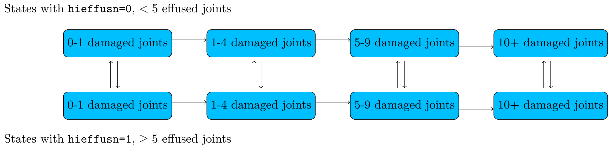
Figure 5.1: Joint model for progression of damage
Then we could predict future outcomes for someone with a particular combination of states and risk factors (= someone in a particular state in the expanded model).
This kind of model can be tricky to deal with due to the large number of parameters - see e.g. Tom and Farewell.
For identifiability / interpretability, may need to constrain some parameters to equal each other using the qconstraint option to msm()
- e.g. we might assume the state of damage doesn’t affect transition rates between effusion states, but the effusion state affects the rates of progression of joint damage. The appropriate assumption depends on the clinical application.
5.4 Time itself as a covariate
Could easily fit a model with the time of the observation as a covariate (months in this example), with a linear effect on the log intensities, e.g.
psor.msm <- msm(state ~ months,
                covariates = ~ months,
                ...
)
Again this assumes that the months covariate is constant between each person’s visit.
But we may want to express a model with
constant intensities within particular time periods (0-6, 6-12 months)
hence the intensity changes for everyone at the same time
To do this, could define a factor (categorical) covariate for the time period, timeperiod say. Then would need to insert an extra observation at the change times (6 and 12 months) for each person with the value of this covariate:
##     ptnum state months timeperiod
## 10      6     1   3.70   [-Inf,6)
## 1.6     6    NA   6.00     [6,12)
## 11      6     1   6.02     [6,12)
## 12      6     2   6.60     [6,12)
## 1.7     6    NA  12.00   [12,Inf)
## 13      6     2  12.52   [12,Inf)
## 14      6     3  13.04   [12,Inf)
## 15      6     3  16.78   [12,Inf)
## 16      6     4  17.28   [12,Inf)
Problem is that the state is unknown at 6 and 12 years if the data are intermittently observed.
We need a new tool to compute the likelihood in this situation…
5.5 Partially-known states
If a state is unknown at a particular time, msm can compute the likelihood as a sum over the potential values of the likelihood given the unknown state.
Replace the NA values in the data for the unknown state with a code (99, say), and use the following syntax to fit the model while telling msm what states this code can represent:
msm(...,
censor = 99,   # code that you gave in the data for the unknown state
censor.states = c(1,2,3,4) # e.g. if code 99 could mean either state 1, 2, 3 or 4
                         # defaults to all non-absorbing states
)
Two common examples
censored survival times when multi-state model includes death as a state. We know someone is alive at the end of the study, but we don’t know their clinical state at this time.
(as in the example here) time-dependent intensities that change at a common time. We know the value of the “time period” covariate, but not the state, at that time.
(Footnote: msm syntax uses the term censor, because a censored random variable is one that is partially observed, but in msm this refers to a partially observed state, not a partially-known event time.)
5.6 pci: piecewise constant intensities (which change at common times)
msm provides a shorthand for these models where the intensities depend on the time period.
Supply the times when all intensities change in the pci argument. msm will automatically construct a categorical covariate indicating the time period, impute artificial observations at the change times, and construct and fit a censor model to calculate and maximise the correct likelihood.
psorpci.msm <- msm(state ~ months, subject = ptnum,
                   data = psor, qmatrix = Q, gen.inits=TRUE,
                   pci = c(5,10))
psorpci.msm
##
## Call:
## msm(formula = state ~ months, subject = ptnum, data = psor, qmatrix = Q, gen.inits = TRUE, pci = c(5, 10))
##
## Maximum likelihood estimates
## Baselines are with covariates set to their means
##
## Transition intensities with hazard ratios for each covariate
## Baseline timeperiod[5,10)
## State 1 - State 1 -0.09001 (-0.11248,-0.07204)
## State 1 - State 2 0.09001 ( 0.07204, 0.11248) 0.8256 (0.4659,1.463)
## State 2 - State 2 -0.16094 (-0.20383,-0.12707)
## State 2 - State 3 0.16094 ( 0.12707, 0.20383) 0.7212 (0.3553,1.464)
## State 3 - State 3 -0.28017 (-0.38534,-0.20370)
## State 3 - State 4 0.28017 ( 0.20370, 0.38534) 0.9398 (0.3507,2.519)
## timeperiod[10,Inf)
## State 1 - State 1
## State 1 - State 2 0.6993 (0.3976,1.230)
## State 2 - State 2
## State 2 - State 3 0.7879 (0.4314,1.439)
## State 3 - State 3
## State 3 - State 4 0.7293 (0.2978,1.786)
##
## -2 * log-likelihood: 1242
## [Note, to obtain old print format, use "printold.msm"]As in any other model with categorical covariates, msm estimates a hazard ratio of transition:
for each category (here, time periods 5-10 and 10+ years),
compared to the baseline category (here, 0-5 years)
No evidence for time dependence in the intensities in this example
5.7 Output functions for models with pci
For models fitted using pci, then the pmatrix.msm and totlos.msm functions will automatically recognise that the model has a covariate representing time since the start of the process.
Here, when we predict the transition probabilities over 15 years, it will automatically adjust for the intensities changing at 5 and 10 years.
So there is no need to use pmatrix.piecewise.msm or supply a covariates argument.
pmatrix.msm(psorpci.msm, t=15)## State 1 State 2 State 3 State 4
## State 1 0.255 0.2067 0.1443 0.394
## State 2 0.000 0.0866 0.1030 0.810
## State 3 0.000 0.0000 0.0144 0.986
## State 4 0.000 0.0000 0.0000 1.000ppass.msm and efpt.msm are not currently supported with time dependent covariates.
5.8 Variants of pci models (advanced)
What if we want to build more detailed models with time-dependent intensities, e.g.
models with a second covariate, whose effect is different within each time period? i.e. a time/covariate interaction.
models where the time period affects some transition intensities but not others?
Construct the expanded dataset
Fit a standard
pcimodel, then usemodel.frame()to extract the expanded dataset constructed bymsm, that hasextra rows at the time change points where the state is unknown,
an automatically-constructed
timeperiodcovariate
psorpci.msm <- msm(state ~ months, subject = ptnum, covariates = ~hieffusn,
                   data = psor, qmatrix = Q, gen.inits=TRUE,
                   pci = c(5,10))
psor_pcidata <- model.frame(psorpci.msm)[,c("(subject)","(state)","(time)",
                                            "timeperiod","hieffusn")]
names(psor_pcidata)[1:3] <- c("ptnum","state","months")
head(psor_pcidata)
## ptnum state months timeperiod hieffusn ## 1 1 1 6.46 [5,10) 0 ## 1.1 1 5 10.00 [10,Inf) 0 ## 2 1 1 17.08 [10,Inf) 0 ## 3 2 1 26.32 [10,Inf) 0 ## 4 2 3 29.48 [10,Inf) 0 ## 5 2 4 30.58 [10,Inf) 0Fit model to the expanded dataset, using
censorThen we can use this dataset for a standard
msmfit withtimeperiodas a categorical covariate.The missing states at the time change points are given a code equal to 1 plus the number of states
- here the “state unknown” code is 5, so call
msmwithcensor = 5.
- here the “state unknown” code is 5, so call
Example (a): Time period only affects the rate of the 1-2 transition:
psorpci.msm <- msm(state ~ months, subject = ptnum,
                   covariates = list("1-2" = ~ timeperiod),
                   data = psor_pcidata,
                   censor = 5,
                   qmatrix = Q, gen.inits=TRUE)
Example (b): Different effect of hieffusn on 1-2 transition rate in each time period
- use the
*operator in the model formula, standard R syntax for interactions in general linear models
psorpci.msm <- msm(state ~ months, subject = ptnum,
                   covariates = list("1-2" = ~ timeperiod*hieffusn),
                   data = psor_pcidata,
                   censor = 5,
                   qmatrix = Q, gen.inits=TRUE)
5.9 Exercises
In the CAV example, investigate how the transition intensities depend on time since transplantation. There is no single correct way to approach this problem - some things that could be done include:
Include years since transplant as a covariate with a linear effect on the log intensities, using the same techniques as in the previous chapter.
Use
pcito fit a model with a categorical “time period” covariate on all intensities.Extract the imputed dataset that
msmconstructs in (2), by usingmodel.frame. Use this dataset to build more refined models with categorical time period variables.
In each case, AIC could be used to compare models with different assumptions about the covariate effect.
Note if you get a numerical overflow error, this may be solved by normalising the optimisation using msm(..., control=list(fnscale=4000)), as described at the end of Chapter 2, noting that the -2 log-likelihood being optimised in this example takes a value of around 4000.
If you get a “iteration limit exceeded” error, use msm(..., control=list(maxit=10000), ...) or some other large number for maxit. This increases the number of iterations that R’s optim function uses before giving up trying to find the maximum.
5.10 Solutions
The following model has a linear effect of time since transplant on all log intensities. The hazards of CAV onset, and the hazards of death in the two CAV states, appear to increase significantly with time.
cav.time.msm <- msm(state ~ years, subject=PTNUM, data=cav, deathexact = TRUE,
                   covariates = ~ years,
                   gen.inits = TRUE, qmatrix=Q_cav,
                   control = list(fnscale=4000, maxit=10000))
cav.time.msm
## ## Call: ## msm(formula = state ~ years, subject = PTNUM, data = cav, qmatrix = Q_cav, gen.inits = TRUE, covariates = ~years, deathexact = TRUE, control = list(fnscale = 4000, maxit = 10000)) ## ## Maximum likelihood estimates ## Baselines are with covariates set to their means ## ## Transition intensities with hazard ratios for each covariate ## Baseline years ## State 1 - State 1 -0.18187 (-0.20833,-0.15877) ## State 1 - State 2 0.14743 ( 0.12546, 0.17325) 1.0984 (1.0444,1.1552) ## State 1 - State 4 0.03444 ( 0.02384, 0.04975) 0.9044 (0.7945,1.0296) ## State 2 - State 1 0.28343 ( 0.20185, 0.39798) 0.8698 (0.7662,0.9875) ## State 2 - State 2 -0.63973 (-0.76405,-0.53564) ## State 2 - State 3 0.31914 ( 0.25390, 0.40115) 0.9940 (0.9180,1.0764) ## State 2 - State 4 0.03716 ( 0.01064, 0.12981) 1.2981 (1.0772,1.5644) ## State 3 - State 2 0.10361 ( 0.04616, 0.23253) 1.1543 (0.8678,1.5355) ## State 3 - State 3 -0.35814 (-0.50226,-0.25538) ## State 3 - State 4 0.25454 ( 0.17571, 0.36872) 1.0525 (0.9439,1.1737) ## ## -2 * log-likelihood: 3922 ## [Note, to obtain old print format, use "printold.msm"]We might simplify this model to include only the effects that appeared to be significant.
cav.timei.msm <- msm(state ~ years, subject=PTNUM, data=cav, deathexact = TRUE,
                   covariates = list("1-2"=~ years, "2-1" = ~years,
                                 "2-4"=~years, "3-4"=~years),
                   gen.inits = TRUE, qmatrix=Q_cav,
                   control = list(fnscale=4000, maxit=10000))
cav.timei.msm
## ## Call: ## msm(formula = state ~ years, subject = PTNUM, data = cav, qmatrix = Q_cav, gen.inits = TRUE, covariates = list(`1-2` = ~years, `2-1` = ~years, `2-4` = ~years, `3-4` = ~years), deathexact = TRUE, control = list(fnscale = 4000, maxit = 10000)) ## ## Maximum likelihood estimates ## Baselines are with covariates set to their means ## ## Transition intensities with hazard ratios for each covariate ## Baseline years ## State 1 - State 1 -0.18614 (-0.211964,-0.16346) ## State 1 - State 2 0.14427 ( 0.122891, 0.16936) 1.0891 (1.034,1.1467) ## State 1 - State 4 0.04187 ( 0.033765, 0.05192) 1.0000 ## State 2 - State 1 0.29050 ( 0.207070, 0.40753) 0.8757 (0.771,0.9944) ## State 2 - State 2 -0.64303 (-0.769194,-0.53756) ## State 2 - State 3 0.32637 ( 0.259889, 0.40986) 1.0000 ## State 2 - State 4 0.02616 ( 0.005242, 0.13058) 1.3016 (1.024,1.6547) ## State 3 - State 2 0.13773 ( 0.083810, 0.22634) 1.0000 ## State 3 - State 3 -0.39177 (-0.528195,-0.29058) ## State 3 - State 4 0.25404 ( 0.174921, 0.36895) 1.0639 (0.967,1.1706) ## ## -2 * log-likelihood: 3927 ## [Note, to obtain old print format, use "printold.msm"]Or go even further and constrain the hazard ratio for time on death from the two CAV states to be the same, as the mechanism for these effects is plausibly the same.
cav.timec.msm <- msm(state ~ years, subject=PTNUM, data=cav, deathexact = TRUE,
                   covariates = list("1-2"=~ years, "2-1"=~years, "2-4"=~years, "3-4"=~years),
                   constraint = list(years = c(1,2,3,3)),
                   gen.inits = TRUE, qmatrix=Q_cav,
                   control = list(fnscale=4000, maxit=10000))
cav.timec.msm
## ## Call: ## msm(formula = state ~ years, subject = PTNUM, data = cav, qmatrix = Q_cav, gen.inits = TRUE, covariates = list(`1-2` = ~years, `2-1` = ~years, `2-4` = ~years, `3-4` = ~years), constraint = list(years = c(1, 2, 3, 3)), deathexact = TRUE, control = list(fnscale = 4000, maxit = 10000)) ## ## Maximum likelihood estimates ## Baselines are with covariates set to their means ## ## Transition intensities with hazard ratios for each covariate ## Baseline years ## State 1 - State 1 -0.18557 (-0.21108,-0.1631) ## State 1 - State 2 0.14434 ( 0.12310, 0.1693) 1.0911 (1.0359,1.1491) ## State 1 - State 4 0.04122 ( 0.03306, 0.0514) 1.0000 ## State 2 - State 1 0.28628 ( 0.20373, 0.4023) 0.8784 (0.7725,0.9988) ## State 2 - State 2 -0.65637 (-0.78170,-0.5511) ## State 2 - State 3 0.32038 ( 0.25459, 0.4032) 1.0000 ## State 2 - State 4 0.04971 ( 0.02258, 0.1095) 1.1209 (1.0441,1.2034) ## State 3 - State 2 0.14035 ( 0.08532, 0.2309) 1.0000 ## State 3 - State 3 -0.35431 (-0.47298,-0.2654) ## State 3 - State 4 0.21396 ( 0.15048, 0.3042) 1.1209 (1.0441,1.2034) ## ## -2 * log-likelihood: 3929 ## [Note, to obtain old print format, use "printold.msm"]AIC(cav.time.msm, cav.timei.msm, cav.timec.msm)## df AIC ## cav.time.msm 14 3950 ## cav.timei.msm 11 3949 ## cav.timec.msm 10 3949An alternative approach is based on discretising time, and defining different effects in different time periods, e.g. before and after 5 years. We could use
pcito fit a model where all intensities have an effect of time period, and then extract the imputed dataset to build more elaborate models of this type.cav.pci5.msm <- msm(state ~ years, subject=PTNUM, data=cav, deathexact=TRUE, pci = c(5), gen.inits = TRUE, qmatrix=Q_cav, control = list(fnscale=4000, maxit=10000)) cav_imp <- model.frame(cav.pci5.msm) names(cav_imp)[1:3] <- c("PTNUM","state","years")To the dataset with values of
yearsandtimeperiodvalues imputed at 5 years, we fit two alternative models, both with a covariate effect on the intensities where the effect was significant (from the non-imputed datasets) and with the effects on death constrained to be the same. One model has a linear effect of a continuous time covariate, and in the other model, this covariate is discretised at 5 years.cav.imp.linear.msm <- msm(state ~ years, subject=PTNUM, data=cav_imp, deathexact=TRUE, covariates = list("1-2"=~years, "2-1"=~years, "2-4"=~years, "3-4"=~years), censor = 5, # the code that msm used for the hidden state, i.e. "state 5" gen.inits = TRUE, qmatrix=Q_cav, control = list(fnscale=4000,maxit=10000)) cav.imp.binary.msm <- msm(state ~ years, subject=PTNUM, data=cav_imp, deathexact=TRUE, covariates = list("1-2"=~timeperiod, "2-1"=~timeperiod, "2-4"=~timeperiod, "3-4"=~timeperiod), censor = 5, gen.inits = TRUE, qmatrix=Q_cav, control = list(fnscale=4000,maxit=10000)) AIC(cav.pci5.msm, cav.imp.linear.msm, cav.imp.binary.msm)## df AIC ## cav.pci5.msm 14 3948 ## cav.imp.linear.msm 11 3946 ## cav.imp.binary.msm 11 3943The model
cav.imp.binary.msmwith time period as a binary effect on selected transitions has a slightly improved AIC over the alternative models.
Note that it might be possible to find even better fitting models than these - but with intermittently-observed data, it is difficult to produce exploratory plots that would indicate what the shape of the dependence on time might be, or what cut-points for time periods might be appropriate.