Part 3 Prediction from multi-state models
Previously we fitted a multi-state model and presented the estimated transition intensities.
Multi-state models describe a process evolving over time. Given that fitted model, we usually want to predict what will happen to a person who follows that model.
This section of the course describes various “predictive” quantities that we could estimate, which are functions of the intensities in the model.
3.1 Mean sojourn time
The mean sojourn time in a state \(r\) is the expected length of one period spent in that state. Recall it is defined as \(-1 / q_{rr}\). Given a fitted model, estimates of the mean sojourn times can be easily extracted using sojourn.msm, with standard errors and confidence intervals.
options(digits=3)
sojourn.msm(psor.msm)
## estimates SE L U
## State 1 10.96 1.228 8.80 13.65
## State 2 6.36 0.733 5.08 7.98
## State 3 3.85 0.501 2.98 4.973.2 Transition probability matrix
Transition probabilities \(P = Exp(t Q)\) over any time interval \(t\) can be calculated, given a fitted model, using pmatrix.msm.
These are continuous-time models, so we have to specify the interval \(t\) we want to predict over. The default is \(t=1\), but this may not be interest. In the psoriatic arthritis example, note how the chance of occupying state 4 goes up rapidly from \(t=1\) to \(t=10\), for every starting state.
pmatrix.msm(psor.msm, t=1)## State 1 State 2 State 3 State 4
## State 1 0.913 0.0806 0.00606 0.000547
## State 2 0.000 0.8546 0.12764 0.017793
## State 3 0.000 0.0000 0.77119 0.228810
## State 4 0.000 0.0000 0.00000 1.000000pmatrix.msm(psor.msm, t=10)## State 1 State 2 State 3 State 4
## State 1 0.402 0.268 0.1397 0.190
## State 2 0.000 0.208 0.2041 0.588
## State 3 0.000 0.000 0.0744 0.926
## State 4 0.000 0.000 0.0000 1.000But where are the standard errors or confidence intervals?
3.3 Characterising uncertainty about functions of intensities
Getting confidence intervals and standard errors for transition probabilites and related quantities is not trivial computationally. Two ways in msm:
ci="normal".Repeatedly draw from the asymptotic sampling distribution of the estimated log intensities (and covariate effects), which is a multivariate normal with mean defined by the maximum likelihood estimates, and covariance defined by the (inverse) Hessian at the maximised log likelihood.
Compute the P matrix for each draw, and obtain the confidence interval from the quantiles of \(B\) samples.
pmatrix.msm(psor.msm, ci="normal", B=100)## State 1 State 2 ## State 1 0.9127936 (0.8950459,0.9276806) 0.0806027 (0.0666926,0.0974142) ## State 2 0 0.8545672 (0.8210479,0.8771882) ## State 3 0 0 ## State 4 0 0 ## State 3 State 4 ## State 1 0.0060564 (0.0045665,0.0080828) 0.0005474 (0.0004027,0.0007505) ## State 2 0.1276400 (0.1078558,0.1555821) 0.0177928 (0.0139712,0.0230815) ## State 3 0.7711897 (0.7138962,0.8135015) 0.2288103 (0.1864985,0.2861038) ## State 4 0 1.0000000 (1.0000000,1.0000000)ci="boot".Repeatedly draw bootstrap resamples of the data, refit the model for each sample, and summarise the estimates over the repeated samples (slower but more accurate, as avoids asymptotic normal approximation)
pmatrix.msm(psor.msm, ci="boot", B=100)
In either method, it is sensible to check \(B\) is large enough, by computing for larger values of \(B\) and checking if the result is stable.
3.4 Total length of stay in states
For someone in state \(r\) now, over the next \(t=10\) years they are expected to spend a total of:
? years in state \(s=1\)
? years in state \(s=2\) …
Defined as \(\int_{0}^{t} P(u)_{rs} du\), for each \(s\), and computed in msm by the totlos.msm function
totlos.msm(psor.msm, t=10)## State 1 State 2 State 3 State 4
## 6.559 2.101 0.733 0.607Note the difference from the mean sojourn time, which only refers to the time of a single period in the current state.
Total length of stay adds up all periods that a person is predicted to spend in a state, both now and in the future.
3.5 Expected first passage time
The expectation of the time until someone currently in state \(r\) next enters a particular state (the “passage” time or “hitting” time) can be computed with efpt.msm. See help(efpt.msm) for the theory behind this.
Here, for people currently in state 1, 2, 3 and 4 respectively, the expected time to state 4 is:
efpt.msm(psor.msm, tostate=4)## [1] 21.17 10.21 3.85 0.00Obviously under this model, the expected time to the severest state, state 4, decreases as the starting state becomes more severe.
3.6 Predicting the prevalence of states over time
“Expected” prevalence of state \(s\) at time \(t\) defined by the transition probabilities from state \(r\) to state \(s\), averaged by the proportion who start in each state \(r\).
Model fit can be checked by comparing the expected prevalence with the observed proportion in the data occupying each state at each time.
plot.prevalence.msm(psor.msm)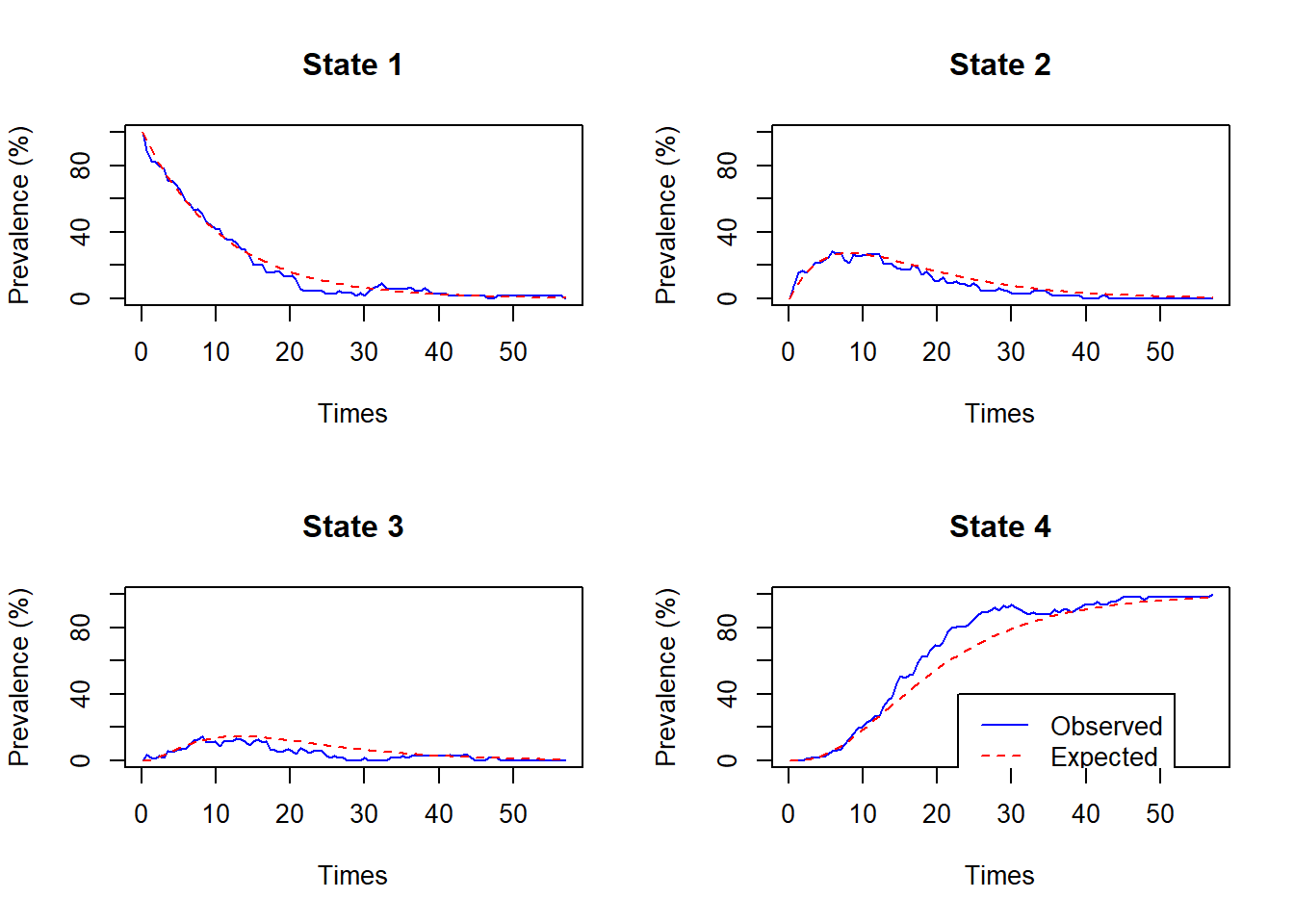
Note that observed prevalence at time \(t\) is not known if people are not all measured at time \(t\), so msm has to estimate this by interpolation. So this check of fit is rough.
3.7 Passage probabilities
For a person in state \(r\) now, this is the probability that before time \(t\), they will visit state \(s\) at least once. Calculated in msm using ppass.msm.
This function works by defining a new model equivalent to the original model, except that state \(s\) is an absorbing state. The passage probability is defined by the transition probabilities to state \(s\) in the new model.
ppass.msm(psor.msm, tot=10)## to
## from State 1 State 2 State 3 State 4
## State 1 1 0.598 0.330 0.190
## State 2 0 1.000 0.792 0.588
## State 3 0 0.000 1.000 0.926
## State 4 0 0.000 0.000 1.000For people in state 1, there is a 1 in 3 chance of experiencing progression to state 3 or worse by 10 years.
In this model, we could have got the same result by adding up the transition probabilities. For example, the passage probability from state 1 to state 3 by 10 years is equal to \(P(t=10)_{13} + P(t=10)_{14}\), since the event “went through state 3 before 10 years” is equivalent to “is in state 3 or state 4 at 10 years”. However that reasoning would not work for a model that allowed transitions back from state 3 to state 2.
P <- pmatrix.msm(psor.msm, t=10)
P[1,3] + P[1,4]
## [1] 0.333.8 Exercises
Using the CAV model that you fitted in the exercises from the previous chapter, investigate how the survival probability depends on the state of CAV.
For a new heart transplant recipient, how likely is it that someone will experience severe CAV before dying?
Does the model appear to fit the data?
Note that if death times are known, you could also check the fit of an
msmmodel by comparing estimated survival probabilities with Kaplan-Meier estimates (in addition to comparing observed and expected prevalence).msmhas a shortcut function to check fitted survival probabilities, called asplot.survfit.msm(x, from=1), wherexis your fitted model, andfromindicates the starting state from which to forecast survival. Look at the help page for this function, and customise the plot to your liking.
3.9 Solutions
Picking a range of prediction times covering those in the data (e.g. 1 year, 5 years, 10 years), we can compute the probability of death (state 4 in the model) by this time by extracting the fourth column of the transition probability matrix.
pmatrix.msm(cav.msm, ci="normal", t=1)[,4]## estimate lower upper ## [1,] 0.0429 0.0362 0.0519 ## [2,] 0.0718 0.0535 0.1402 ## [3,] 0.2519 0.2054 0.3087 ## [4,] 1.0000 1.0000 1.0000pmatrix.msm(cav.msm, ci="normal", t=5)[,4]## estimate lower upper ## [1,] 0.251 0.225 0.293 ## [2,] 0.436 0.384 0.537 ## [3,] 0.701 0.624 0.784 ## [4,] 1.000 1.000 1.000pmatrix.msm(cav.msm, ci="normal", t=10)[,4]## estimate lower upper ## [1,] 0.505 0.468 0.564 ## [2,] 0.685 0.635 0.761 ## [3,] 0.865 0.808 0.914 ## [4,] 1.000 1.000 1.000At each time, the risk of death by this time increases sharply with the severity of CAV.
These risks are high, but note that the data only include outcomes without treatment. In practice, people who are diagnosed with CAV will get treatment (e.g. coronary artery revascularisation). Outcomes after treatment were excluded from the
cavdata.We can calculate the passage probability from state 1 (no CAV) to state 3 (severe CAV) for a very high time interval, and check that the result does not change if an even higher time interval is supplied. (a finite number must be supplied –
tot=Infwill not work)ppass.msm(cav.msm, tot=100)["State 1","State 3"]## [1] 0.586ppass.msm(cav.msm, tot=1000)["State 1","State 3"]## [1] 0.586pp <- ppass.msm(cav.msm, tot=100, ci="normal") pp[1,3]## estimate lower upper ## 0.586 0.459 0.654Judging from the comparison of observed and predicted prevalences, and comparing with the Kaplan-Meier survival estimates, the model appears to underestimate the probability of death at later times.
plot.prevalence.msm(cav.msm)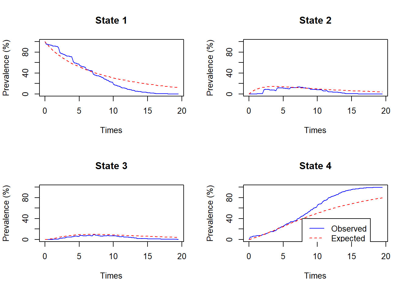
plot.survfit.msm(cav.msm, from=1,
                 ylab="Survival probability",
                 xlab="Time after transplant",
                 col="red",
                 col.surv="black")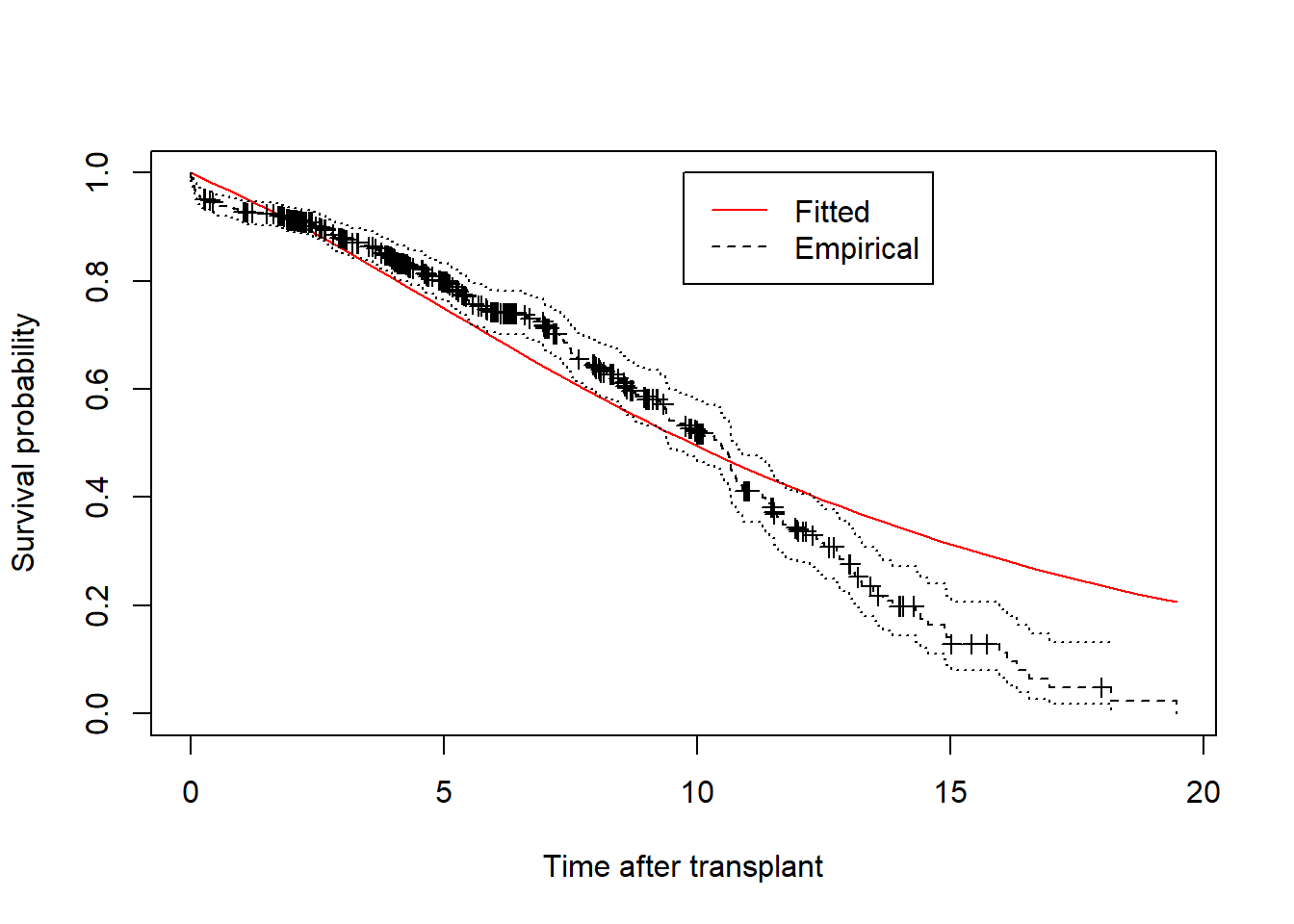
In fact (though you were not expected to know this from the information given in the question!) this is an artefactual finding resulting from people in the data being followed up for different lengths of time. To calculate the probability at each time,
msmuses a denominator defined by the number of people whose state we know at this time. This overestimates the probability of death, because the people whose state we know at later times are more likely to be the people who have died. We don’t know the state at later times for people whose outcomes were censored at the end of the study when they were still alive.We could correct for this bias if we impose an “end of study” time for every person, and exclude people from the denominator after this time, even people who we know to have died. These can be supplied as the
censtimeargument toplot.prevalence.msm, but these times are not available in thecavdataset supplied withmsm.