Part 4 msm models with covariates
4.1 Reminder of covariates in multi-state models
The intensity for each \(r-s\) transition can be expressed as a log-linear function of covariates, denoted as a vector \(\mathbf{z}\).
\[q_{rs} = q_{rs}^{(0)} \exp(\boldsymbol{\beta}_{rs}^{\prime} \mathbf{z})\] Psoriatic arthritis example: investigate risk factors for joint damage
psor data contains two covariates:
hieffusn: Five or more effused jointsollwsdrt: Low erythrocyte sedimentation rate (less than 15 mm/h)
Each row of the data contains value for that person at study entry (people just diagnosed), so covariate values are the same throughout each person’s follow-up.
head(psor, 5)## ptnum months state hieffusn ollwsdrt
## 1 1 6.46 1 0 1
## 2 1 17.08 1 0 1
## 3 2 26.32 1 0 0
## 4 2 29.48 3 0 0
## 5 2 30.58 4 0 04.2 Choices for modelling covariates
There are three transitions in the model. Which transitions should be affected by which covariates?
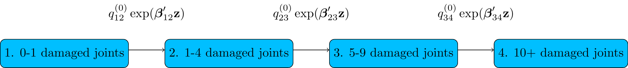
Figure 4.1: Psoriatic arthritis
Don’t just put all covariates on all transitions without thinking — you may not have enough data informing transitions out of particular states.
statetable.msm(state, ptnum, data=psor)## to
## from 1 2 3 4
## 1 183 56 16 8
## 2 0 100 35 18
## 3 0 0 48 37With 37 transitions, for example, unlikely to get usefully-precise effect estimates for 10 covariates on the State 3 - State 4 transition rate, but 3 covariates may be feasible.
No shrinkage / penalized likelihood methods implemented in msm unfortunately, but standard variable selection methods, e.g. AIC, are simple to implement, as we will see.
4.3 msm syntax: covariates on rates of specific transitions
Use the covariates argument to msm to place covariates on transition intensities.
Set covariates to a list of linear model formulae, named by the transition, to specify which intensities get which covariates.
psorc_spec.msm <- msm(state ~ months,
                  subject = ptnum,
                  data = psor,
                  qmatrix = Q,
                  covariates = list("1-2" = ~ hieffusn,
                                    "2-3" = ~ hieffusn + ollwsdrt),
                  gen.inits=TRUE)
4.4 Covariates on all transition rates
To put the same covariates on all the transition rates, can set the covariates argument to a single
formula (instead of a list of formulae).
psorc_all.msm <- msm(state ~ months,
                     subject = ptnum,
                     data = psor,
                     qmatrix = Q,
                     covariates = ~ hieffusn + ollwsdrt,
                     gen.inits=TRUE)
4.5 Identical effects of same covariate on different transitions
constraint argument: a list with one named element for each covariate with constrained effects, so that the hazard ratio for that covariate is the same for different transitions.
Each list element is a vector of integers, of same length as the number of transition rates.
Which elements of this vector are the same determines which covariate effects are assumed to be equal.
In this model, the effect of hieffusn is the same for the first two transition rates, i.e. the progression rates from State 1 to 2 and from State 2 to 3, but different for the State 3 - 4 rate
psorc_cons.msm <- msm(state ~ months,
                subject = ptnum,
                data = psor,
                qmatrix = Q,
                covariates = ~ hieffusn + ollwsdrt,
                constraint = list(hieffusn = c(1,1,2)),
                gen.inits=TRUE)
4.6 Covariate selection
Compare the three different models above using Akaike’s information criterion (AIC = -2\(\times\)log likelihood + 2*df), where “df” is the number of estimated parameters (degrees of freedom). AIC is an approximate measure of the predictive ability of a model.
There is not much difference, but the model with the lowest AIC is psorc_spec.msm with different predictors on specific transitions.
logliks <- c(logLik(psorc_spec.msm), logLik(psorc_cons.msm), logLik(psorc_all.msm))
AICs <- AIC(psorc_spec.msm, psorc_cons.msm, psorc_all.msm)
cbind(logliks, AICs)
## logliks df AIC
## psorc_spec.msm -558 6 1128
## psorc_cons.msm -557 8 1129
## psorc_all.msm -556 9 1131Most complex model psorc_all.msm has highest log-likelihood, but the extra parameters do not lead to better predictive performance
It seems sufficient to assume that hieffusn is a predictor of the 1-2 and 2-3 transitions, and ollwsdrt is a predictor of the 2-3 transition
Check the coefficients from the fitted models to verify that this is plausible…
4.7 Interpretation of the hazard ratio
Hazard ratios represent how the instantaneous risk of making a particular transition is modified by the covariate. Here, someone in state 1, with 5 or more effused joints (hieffusn=1), is at over twice the risk of progression to state 2, at any time, compared to someone with 4 or fewer (hieffusn=0).
print(psorc_all.msm, digits=2)##
## Call:
## msm(formula = state ~ months, subject = ptnum, data = psor, qmatrix = Q, gen.inits = TRUE, covariates = ~hieffusn + ollwsdrt)
##
## Maximum likelihood estimates
## Baselines are with covariates set to their means
##
## Transition intensities with hazard ratios for each covariate
## Baseline hieffusn ollwsdrt
## State 1 - State 1 -0.10 (-0.127,-0.079)
## State 1 - State 2 0.10 ( 0.079, 0.127) 2.3 (1.09,5.0) 0.73 (0.43,1.26)
## State 2 - State 2 -0.16 (-0.206,-0.128)
## State 2 - State 3 0.16 ( 0.128, 0.206) 1.7 (0.95,3.0) 0.46 (0.26,0.79)
## State 3 - State 3 -0.26 (-0.350,-0.195)
## State 3 - State 4 0.26 ( 0.195, 0.350) 1.4 (0.77,2.5) 1.58 (0.78,3.19)
##
## -2 * log-likelihood: 1113
## [Note, to obtain old print format, use "printold.msm"]Can also extract with
hazard.msm(psorc_all.msm)## $hieffusn
## HR L U
## State 1 - State 2 2.34 1.094 5.00
## State 2 - State 3 1.68 0.950 2.98
## State 3 - State 4 1.39 0.774 2.51
##
## $ollwsdrt
## HR L U
## State 1 - State 2 0.732 0.426 1.258
## State 2 - State 3 0.458 0.264 0.793
## State 3 - State 4 1.576 0.778 3.1934.8 Outputs for different covariate values
Comparing absolute outcomes between groups can be easier to interpret than hazard ratios.
Most of msm’s prediction functions (totlos.msm, ppass.msm, etc.) take an argument called covariates, a list that defines the covariate values to calculate the output for.
Example: probability of transition from state 1 to severest state 4 by 10 years, compared between combinations of risk factors
covariates argument indicates the covariate values \(\mathbf{z}\) to calculate the transition probabilities for.
msm will calculate \(P(t | \hat{q}, \hat\beta, \mathbf{z})\) where \(\hat{q},\hat\beta\) are the fitted baseline intensities and covariate effects.
p00 <- pmatrix.msm(psorc_spec.msm, t=10, covariates=list(hieffusn=0,ollwsdrt=0),
                   ci="normal", B=100)
p01 <- pmatrix.msm(psorc_spec.msm, t=10, covariates=list(hieffusn=0,ollwsdrt=1),
                   ci="normal", B=100)
p10 <- pmatrix.msm(psorc_spec.msm, t=10, covariates=list(hieffusn=1,ollwsdrt=0),
                   ci="normal", B=100)
p11 <- pmatrix.msm(psorc_spec.msm, t=10, covariates=list(hieffusn=1,ollwsdrt=1),
                   ci="normal", B=100)
p_14 <- rbind(p00[1,4], p01[1,4], p10[1,4], p11[1,4])
Low sedimentation rate is protective (lower transition probabilities for ollwsdrt=1), while high effusion is a risk factor for progression (higher transition probabilities for hieffusn=1)
cbind(hieffusn = c(0,0,1,1), ollwsdrt=c(0,1,0,1), p_14)## hieffusn ollwsdrt estimate lower upper
## [1,] 0 0 0.205 0.1500 0.270
## [2,] 0 1 0.120 0.0855 0.178
## [3,] 1 0 0.484 0.2922 0.688
## [4,] 1 1 0.324 0.1866 0.4994.9 Exercises
We want to investigate whether heart transplant recipients who have previously had ischaemic heart disease are more at risk of CAV, which is a similar condition. The “primary diagnosis” (reason for having a heart transplant) is included in the CAV data in the categorical variable pdiag, which takes the value IHD for ischaemic heart disease.
Convert this to a binary variable, and develop a multi-state model like the one you built in the previous chapters, including this binary covariate on all transitions.
Adapt the model appropriately so that the covariate is only included on transitions which the covariate is predictive of.
Investigate and compare with a model where the effect of this covariate is constrained to be the same between different transitions.
Compare the clinical prognosis for people with and without pre-transplant IHD, using outcomes similar to those calculated in the previous chapter.
(Note: if calculating the observed and expected prevalences for a subset of patients, then a
subsetargument toplot.prevalence.msmshould be specified. This should be set to a vector of the unique patient IDs included in the appropriate subset.)
4.10 Solutions
We convert the categorical variable
pdiagto a binary 0/1 covariate indicating primary diagnosis of IHD. First we fit the full model where the binary covariate affects all transitions, and examine the hazard ratios under this model.cav$IHD <- as.numeric(cav$pdiag == "IHD") cavcov.msm <- msm(state ~ years, subject=PTNUM, data=cav, covariates = ~IHD, deathexact = TRUE, gen.inits = TRUE, qmatrix=Q_cav) cavcov.msm## ## Call: ## msm(formula = state ~ years, subject = PTNUM, data = cav, qmatrix = Q_cav, gen.inits = TRUE, covariates = ~IHD, deathexact = TRUE) ## ## Maximum likelihood estimates ## Baselines are with covariates set to their means ## ## Transition intensities with hazard ratios for each covariate ## Baseline IHD ## State 1 - State 1 -0.17057 (-0.19084,-0.15246) ## State 1 - State 2 0.12845 ( 0.11159, 0.14785) 1.5279 (1.15331, 2.024) ## State 1 - State 4 0.04212 ( 0.03365, 0.05274) 1.4870 (0.94878, 2.331) ## State 2 - State 1 0.22974 ( 0.17089, 0.30885) 0.9270 (0.51291, 1.675) ## State 2 - State 2 -0.61327 (-0.71676,-0.52472) ## State 2 - State 3 0.34288 ( 0.27220, 0.43191) 0.9633 (0.60716, 1.528) ## State 2 - State 4 0.04065 ( 0.01130, 0.14623) 0.9333 (0.07213,12.076) ## State 3 - State 2 0.13300 ( 0.08069, 0.21922) 0.7380 (0.27167, 2.005) ## State 3 - State 3 -0.44500 (-0.56314,-0.35165) ## State 3 - State 4 0.31200 ( 0.24218, 0.40196) 0.7412 (0.44660, 1.230) ## ## -2 * log-likelihood: 3925 ## [Note, to obtain old print format, use "printold.msm"]We see that the pre-transplant IHD is associated with an increased risk of CAV onset (state 1 - state 2), and possibly also with death before CAV onset (state 1 - state 4). The confidence intervals for the hazard ratios of IHD on the other transition rates are wide and include the null 1.
Hence we build a simplified model, in which IHD only affects the transition rates out of State 1. This model has an improved AIC compared to the bigger model, despite having 5 fewer parameters (
df).cavcov1.msm <- msm(state ~ years, subject=PTNUM, data=cav, covariates = list("1-2"=~IHD, "1-4"=~IHD), deathexact = TRUE, gen.inits = TRUE, qmatrix=Q_cav) AIC(cavcov.msm, cavcov1.msm)## df AIC ## cavcov.msm 14 3953 ## cavcov1.msm 9 3945The hazard ratios for IHD on the risk of CAV onset and pre-CAV death appear to be similar, so we might constrain them to be equal, as follows. The AIC is slightly smaller than for the model where these effects are different.
cavcov2.msm <- msm(state ~ years, subject=PTNUM, data=cav,
                   covariates = list("1-2"=~IHD, "1-4"=~IHD),
                   constraint = list(IHD = c(1,1)),
                   deathexact = TRUE, gen.inits = TRUE, qmatrix=Q_cav)
AIC(cavcov2.msm)
## [1] 3943However despite the statistical improvement, this model would not be clinically meaningful if pre-transplant IHD affects the risk of CAV onset and death after CAV through different mechanisms. We would then prefer to acknowledge that the true effects might be different.
We could compare the transition probabilities at a future time (e.g. 5 years after transplant) for people with and without pre-transplant IHD. The risk of occupying any of the CAV states at this time, and the risk of death by this time, is about 50% more for people with previous IHD, while the chance of being CAV-free (state 1) is correspondingly lower.
pmatrix.msm(cavcov.msm, t=5, covariates=list(IHD=0))## State 1 State 2 State 3 State 4 ## State 1 0.5884 0.1197 0.0703 0.222 ## State 2 0.2747 0.1273 0.1459 0.452 ## State 3 0.0716 0.0647 0.1264 0.737 ## State 4 0.0000 0.0000 0.0000 1.000pmatrix.msm(cavcov.msm, t=5, covariates=list(IHD=1))## State 1 State 2 State 3 State 4 ## State 1 0.4494 0.1571 0.114 0.280 ## State 2 0.2189 0.1483 0.210 0.423 ## State 3 0.0537 0.0712 0.207 0.668 ## State 4 0.0000 0.0000 0.000 1.000The passage probability to severe CAV (which we computed in the previous chapter), i.e. the chance of going through the “severe CAV” state before death, is similar between both groups of people (
IHD=0) and (IHD=1), though slightly higher for people who have had IHD.ppass.msm(cavcov1.msm, tot=100, covariates=list(IHD=0))["State 1","State 3"]## [1] 0.574ppass.msm(cavcov1.msm, tot=100, covariates=list(IHD=1))["State 1","State 3"]## [1] 0.595We might also compare the total length of stay in each state over a long time horizon (e.g. 20 years), finding that people who had IHD are expected to spend longer periods of time in the CAV states (2 and 3) and die sooner.
totlos.msm(cavcov1.msm, tot=20, covariates=list(IHD=0))## State 1 State 2 State 3 State 4 ## 8.80 1.66 1.21 8.33totlos.msm(cavcov1.msm, tot=20, covariates=list(IHD=1))## State 1 State 2 State 3 State 4 ## 6.47 1.96 1.45 10.11The expected times from state 1 to death (
tostate=4) in the two groups can be compared as follows. These are shorter for people who have had IHD.efpt.msm(cavcov1.msm, tostate=4, covariates=list(IHD=0), ci="normal")[,1]## est 2.5% 97.5% ## 14.8 12.5 16.9efpt.msm(cavcov1.msm, tostate=4, covariates=list(IHD=1), ci="normal")[,1]## est 2.5% 97.5% ## 11.26 9.74 12.60Let’s also compare the observed and expected prevalences. Note the use of the
subsetargument to restrict the observed prevalences to those observed in the indicated set of patient IDs.notihd_pts <- unique(cav$PTNUM[cav$IHD==0]) ihd_pts <- unique(cav$PTNUM[cav$IHD==1]) plot.prevalence.msm(cavcov.msm, covariates=list(IHD=0), subset=notihd_pts)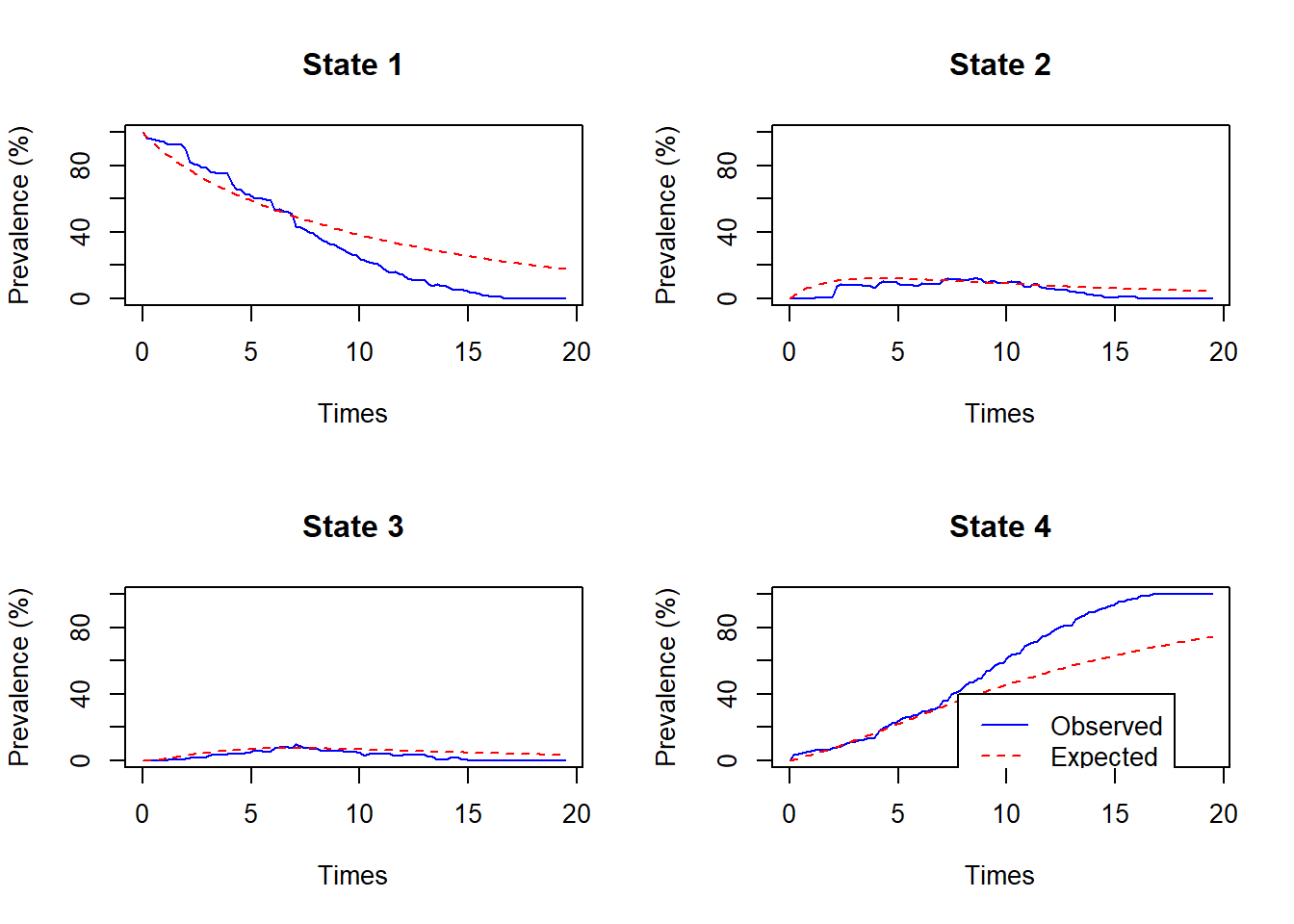
plot.prevalence.msm(cavcov.msm, covariates=list(IHD=1), subset=ihd_pts)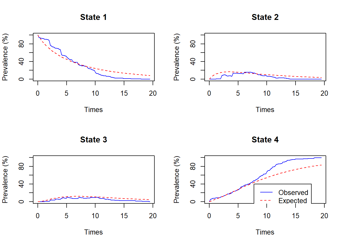
If desired, the function
prevalence.msmcould be used to extract the numbers behind the plots shown byplot.prevalence.msm, to enable multiple groups to be shown on the same plot, or to produce other customised plots.