Priors in survextrap models

The flexible survival models in survextrap are Bayesian.

This means that they analyse data under a parametric model, which assumes that each data point \(x\) comes from a sampling distribution with probability density function \(f(x|\theta)\). The parameters \(\theta\) are estimated by combining a prior distribution \(p(\theta)\), representing beliefs about model parameters external to the data, with a “likelihood” that represents the information from a set of data \(\boldsymbol{x}\), producing a posterior distribution \(p(\theta | \boldsymbol{x})\).

The principle behind the package is that any information that is relevant to extrapolation should be represented transparently. This is arguably clearest if expressed through data or parametric mechanisms.

Data x include individual-level, right-censored survival data, and aggregate counts of survivors, as described on the front page. Expert judgements about survival can be converted to pseudo-data in the form of aggregate counts.
Parametric mechanisms denote the form of \(f()\). These might include the notion that some people are cured (mixture cure models), or that disease-specific and background hazards can be modelled additively (relative survival models). Conventional parametric survival models (like the Weibull and log-logistic) are generally used out of familiarity, not because they are thought to represent meaningful mechanisms for survival.

The default parametric model in survextrap is a flexible spline-based model. This is designed as a “black box”, which aims to fit the data as well as possible. It is not designed to be treated as a mechanism for extrapolation.

However, this spline model has parameters \(\theta\), which still need prior distributions, because the model is Bayesian!

This article describes these two kinds of “prior” judgements that can be used in survextrap models.

Judgements about survival probabilities, that can be converted to pseudo-data, and treated as part of the model likelihood for data \(\boldsymbol{x}\).
Priors on parameters \(\theta\) in spline models.

Converting prior judgements about survival to external data

We suppose there is some expert judgement about survival over the time period from \(t\) to \(u\), and we can “elicit” this as the probability \(p\) that a person who is alive at \(t\) will have died before \(u\).

This elicitation might be done in many ways (e.g. through consensus methods, or consulting multiple experts and aggregating their beliefs). survextrap does not include tools or guidance for doing elicitation, but further info is available, e.g. from Bojke et al., or SHELF.

One simple way is to elicit:

a best guess for what \(p\) is. We could interpret this as the median of the prior distribution.
upper and lower prior credible limits, such that we are (for example) 90% sure that \(p\) is within this range. We can interpret these as the 5% and 95% quantiles.

As an example, suppose we elicited a best guess of 0.6, and a 90% credible interval of 0.4 to 0.8. These can be fitted to a probability distribution representing beliefs about \(p\). The SHELF R package provides a useful function, fitdist, to do this. We use this to fit a Beta distribution, a typically-used distribution for probabilities.

library(SHELF)
p <- c(0.4, 0.6, 0.8)
bet <- fitdist(vals=p, probs=c(0.05, 0.5, 0.95), lower=0, upper=1)$Beta
bet

##     shape1  shape2
## 1 9.190895 6.19854

This gives a Beta(9.2, 6.2) distribution. We can plot its probability density function, to check that the distribution represents the beliefs about \(p\) that we intended to use:

library(ggplot2)
ggplot(data.frame(p = c(0, 1)), aes(x = p)) +
  stat_function(fun = dbeta, args=list(shape1=bet$shape1, shape2=bet$shape2)) +
  ylab("Density")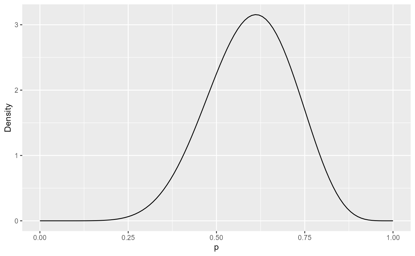

We now convert the elicited Beta distribution to pseudo-data.

The trick for doing this comes from a basic result about Bayesian estimation of an event probability \(p\). Suppose we start with a Beta\((a,b)\) prior for \(p\), and observe \(y\) events out of \(n\) individual observations, where each observation may or may not have resulted in an event, so that \(y\) comes from a Binomial distribution with probability \(p\). The posterior for \(p\) is then Beta\((a+y, b+n-y)\).

We can then equate our elicited belief (call it Beta\((e_1, e_2)\), say) with a posterior distribution under a vague prior (say a Beta\((a=0,b=0)\)). Therefore \(e_1=a+y\) and \(e_2 = b+n-y\), hence \(y=e_1\), \(n = e_1 + e_2\).

In other words, our elicited Beta\((e_1,e_2)\) distribution is equivalent to the knowledge from an aggregate count of \(e_1\) events out of \(e_1 + e_2\) observations. This aggregate “pseudo-data” can be used as an external data source in survextrap.

For example, the Beta(9,6) distribution above is equivalent to pseudo-data of 9 events out of 15 trials. The point estimate of the event probability from this data would be 9/15 = 0.6 (our original guess). A pseudo-dataset of 90 events out of 150 trials would have the same median, but a narrower credible interval, since the dataset is larger, implying greater confidence that the true \(p\) is near to the point estimate.

Further notes on elicitation

Academic note: there are different ways of defining a vague Beta prior for a probability. Beta\((0,0)\) is a uniform distribution for the log odds \(\log(p/(1-p))\), and Beta\((1,1)\) is uniform on the scale of the probability \(p\). The “Jeffreys” prior Beta\((0.5, 0.5)\) is sometimes used as a compromise between these. The difference between these choices is unlikely to matter in practice.
We could elicit survival probabilities over different time intervals, and use these as multiple external datasets in survextrap.
It would probably not be appropriate to include beliefs about the same quantity, elicited from multiple experts, as multiple external datasets in survextrap. This is because the experts may have shared beliefs based on their common knowledge of the field. If multiple experts are consulted about the same quantity, their beliefs should be aggregated into a single distribution before using survextrap, e.g. by using mathematical aggregation or a consensus method. Again, see, e.g. Bojke et al. or SHELF, for more information about elicitation.

Priors on spline parameters

The parameters of the spline model are mathematical abstractions which do not have meaningful interpretations such as means or variances for survival times. However for Bayesian modelling, we still have to place priors on them.

A general way to ensure that the chosen priors represent meaningful beliefs is through simulation. survextrap provides some tools for this.

Plotting plausible hazard trajectories

Before fitting a model, we can use the prior_sample_hazard function to check that hazard curves simulated from the prior would be considered plausible representations of the knowledge that exists outside the data.

To use this before the model is fitted, we have to know the knots defining the spline, and choose a set of priors. survextrap provides a set of default priors, which may or may not be sensible in a given application. and a procedure for picking knots (see the methods vignette).

First we fit a default model, and print the default priors that are used.

library(survextrap)
nd_mod <- survextrap(Surv(years, status) ~ 1, data=colons, fit_method="opt")

print_priors(nd_mod)

## Priors:
##   Baseline log hazard scale: normal(location=0,scale=20)
##   Smoothness SD: gamma(shape=2,rate=1)

The “baseline log hazard scale” parameter is the parameter \(\log(\eta)\) in the definition of the M-spline function for the hazard: \(h(t) = \eta \sum_k p_k b_k(t)\). By itself, \(\eta\) does not define a hazard. It only defines a hazard after being combined with the basis coefficients \(p_k\) and basis terms \(b_k()\).

The “smoothness SD” is the parameter \(\sigma\) . This is even harder to interpret than \(\eta\). Values of \(\sigma=0\) represent certainty that the hazard is the one defined by the prior mean for the \(p_k\). Values of 1 or more favour wiggly hazard curves, while very high values are not meaningful.

The prior mean for the \(p_k\) can be examined in coefs_mean - by default, this defines a hazard function \(h(t)\) that is constant over time. The number and location of knots can also be examined in the mspline component of the model.

round(nd_mod$coefs_mean,2)
sp <- nd_mod$mspline

Together, these knots and prior choices define the model to be fitted to the data. We can now simulate the consequences of these choices, in terms of:

the typical level of the hazard
what range of hazard trajectories are plausible
how much the hazard tends to vary through time

The fitted model object (nd_mod here) has a component called prior_sample, which is a list of functions that can be used to simulate various interesting quantities from this prior specification.

Constant hazard level

The first thing to verify is the typical level of the hazard. If no prior for the hazard scale parameter \(\eta\) is supplied in survextrap, then a default \(N(0,20)\) is used, which is very vague. We can illustrate the implications of this choice by deriving the prior for the constant hazard \(h(t) = \eta \sum_k p_k b_k(t)\) which is implied by the prior for \(\eta\) and the special values of \(p_k\) that imply a constant hazard (found using mspline_constant_coefs()).

The haz_const function returns a summary of the implied prior for this constant hazard, and the implied prior for the mean survival time \(1/h(t)\).

nd_mod$prior_sample$haz_const()

##                haz         mean
## 2.5%  8.336083e-18 1.073931e-17
## 50%   8.810345e-01 1.135029e+00
## 97.5% 9.311588e+16 1.199604e+17

These credible limits are extreme. Perhaps this is reasonable if the dataset is large and would dominate any choice of prior. In most applications, however, we have some idea of what a typical survival time should be, hence what a typical hazard should be, say within an order or two of magnitude.

A simple heuristic is to specify

a prior guess (e.g. we guess that average survival time is 50 years after the start of the study)
a prior upper credible limit (e.g. we guess it is unlikely that the mean survival time is 80 years after the start of the study). Note that this represents uncertainty about the mean survival in a population, rather than the variability between individuals in the population, so perhaps the credible interval should be narrower than you think.
hence giving a median and lower credible limit for \(h(t)\), hence (after dividing by the constant \(\sum_k p_k b_k(t)\) for an arbitrary \(t\) and logging), giving a median \(m\) and lower credible limit \(L\) for \(\log(\eta)\). Hence a normal prior for \(\log(\eta)\) can be defined with median \(m\), and standard deviation \((L-m)/2\).

This is implemented in the function p_meansurv. Note that a spline knot specification is required to obtain the constant \(\sum_k p_k b_k(t)\).

p_meansurv(median=50, upper=80, mspline=sp)

For a given prior on \(\eta\) and spline specification, the function prior_haz_const can be used to summarise the implied prior on the constant hazard and mean survival time. We use this now to check that the prior that we defined with p_meansurv is the one that we intended to define.

prior_haz_const(mspline=sp, 
                prior_hscale = p_meansurv(median=50, upper=80, mspline=sp))

##          haz  mean
## 2.5%  0.0125 31.25
## 50%   0.0200 50.00
## 97.5% 0.0320 80.00

The prior median and upper credible limit match the numbers that we put in. We also get a lower 2.5% credible limit as a consequence of the normal assumption - this should be checked for plausibility, and the prior revised if necessary.

Finally, an updated survextrap model can be fitted that includes the weakly informative prior that we defined and checked. For reporting purposes, we can use print_priors to view the normal prior for \(\log(\eta)\) that was automatically derived.

ndi_mod <- survextrap(Surv(years, status) ~ 1, data=colons, fit_method="opt",
                      prior_hscale = p_meansurv(median=50, upper=80, mspline=sp))
print_priors(ndi_mod)

## Priors:
##   Baseline log hazard scale: normal(location=-3.7853644873736,scale=0.2398021764446)
##   Smoothness SD: gamma(shape=2,rate=1)

Hazard as a function of time

The prior_sample component includes a function called haz which simulates a desired number of hazard trajectories over time, given the prior. This function returns a data frame (here called haz_sim) which contains the hazard value haz, time point time and simulation replicate rep.

Here we simulate nsim=30 prior hazard trajectories from the model ndi_mod, and plot them with ggplot.

set.seed(1)
haz_sim <- ndi_mod$prior_sample$haz(nsim=30)
ggplot(haz_sim, aes(x=time, y=haz, group=rep)) + 
  geom_line() + xlab("Years") + ylab("Hazard") + ylim(0,0.05)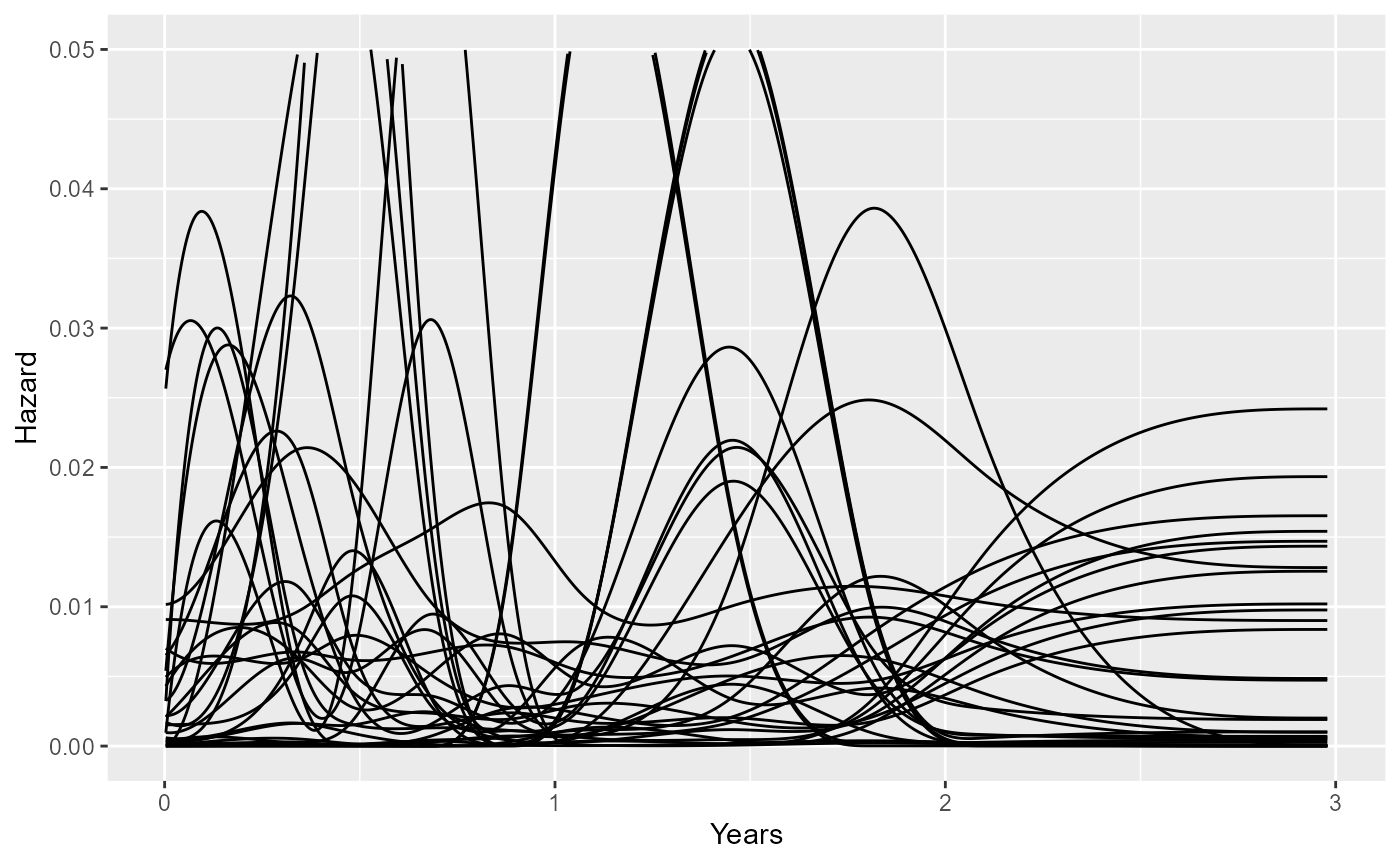

An alternative way is to use the prior_sample_hazard function, which does not require a model to be specified with the survextrap function, but does require the knots and priors to be supplied explicitly.

set.seed(1)
haz_sim <- prior_sample_hazard(knots=sp$knots, degree=sp$degree, 
                               coefs_mean = ndi_mod$coefs_mean,   
                               prior_hsd = p_gamma(2,1),   
                               prior_hscale = p_meansurv(median=50, upper=80, mspline=sp),
                               tmax=3, nsim=30)

These plots can give some idea of how much risks might be expected to vary over time. The parameter driving these variations is \(\sigma\), whose prior can be defined with the prior_hsd argument to survextrap. In the standard survextrap model, \(\sigma=0\) means that we are sure that the hazard will be constant. Therefore we might want to define the prior for \(\sigma\) to rule out implausibly large changes. For example, a Gamma(2,20):

set.seed(1)
haz_sim <- prior_sample_hazard(knots=sp$knots, degree=sp$degree, 
                               coefs_mean = ndi_mod$coefs_mean,   
                               prior_hsd = p_gamma(2,20),   
                               prior_hscale = p_meansurv(median=50, upper=80, mspline=sp),
                             tmax=3, nsim=30)
ggplot(haz_sim, aes(x=time, y=haz, group=rep)) + 
  geom_line() + xlab("Years") + ylab("Hazard") + ylim(0,0.05)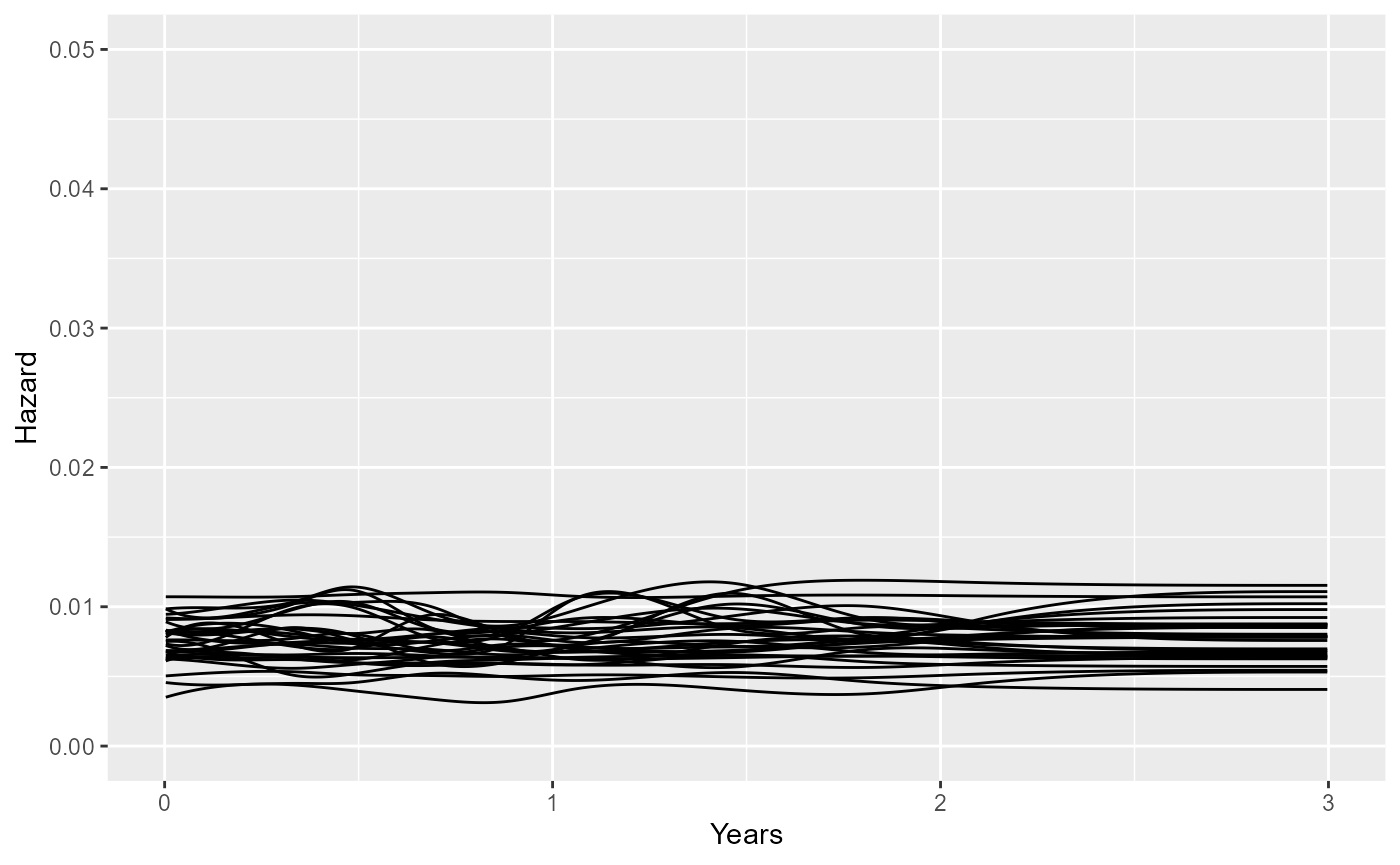

The choice of this prior might be important if we want to extrapolate outside the data, while accounting for potential hazard changes outside the data. If the data informing extrapolation are weak, then the extrapolations will be sensitive to the prior for these potential hazard changes.

Plotting multiple trajectories gives a rough idea of the typical amount of variation through time, but , but ideally we want a more quantitative summary of this.

Ratio between high and low hazards over time

The variation in a hazard curve can be summarised simply by taking a fine grid of equally-spaced points between the time boundary knots, and computing the empirical standard deviation of the hazard on those points. If the hazard is constant, then the SD will be zero.

Since the SD depends on the scale of the hazard, a more useful measure of variation would be the ratio between a particularly high and a particularly low hazard on this grid. High and low might be defined from the 90% and 10% quantiles over time. If the hazard is constant, over time, this ratio will be 1.

These measures are computed by the haz_sd() function: the sd_haz component is the SD over time of the hazard, sd_mean is the SD over time of the inverse hazard, and hr is the high/low hazard ratio (90%/10% by default).

set.seed(1)
ndi_mod$prior_sample$haz_sd()

##            sd_haz      sd_mean           hr
## 2.5%  0.001515510 3.114473e+01 1.817126e+00
## 50%   0.008722217 6.809896e+02 4.013356e+01
## 97.5% 0.024717065 8.197922e+11 4.182825e+08

This shows that the default Gamma\((a=2,b=1)\) prior used in this model is very vague. We can make it less vague by reducing \(a/b\). A Gamma(2, 5), for example, leads to an upper 90% credible limit of about 5 for the hazard ratio over time. Trial and error is probably necessary to produce a prior that is judged plausible by this metric.

set.seed(1)
prior_haz_sd(mspline=sp,                              
             prior_hsd = p_gamma(2,5),   
             prior_hscale = p_meansurv(median=50, upper=80, mspline=sp), 
             quantiles = c(0.1, 0.5, 0.9),
             nsim=1000)

##           sd_haz    sd_mean       hr
## 10% 0.0004542116   9.037567 1.080665
## 50% 0.0018053422  37.800321 1.517070
## 90% 0.0050991490 231.092233 4.620972

Note that a large number of simulations nsim from the prior may be required for a precise estimate of these tail quantiles, and the distribution is skewed, so that the 95% credible limit may be much higher than the 90% limit, for example.

Let us now fit a model and compare the posterior 95% credible interval for this hazard ratio to the prior. The posterior interval is narrower than the prior interval, showing the influence of the data.

library(dplyr)
nd_mod <- survextrap(Surv(years, status) ~ 1, data=colons, fit_method="mcmc",
                     chains=1, iter=1000,
                     prior_hsd = p_gamma(2,5))
qgamma(c(0.025, 0.975), 2, 5)
summary(nd_mod) %>% filter(variable=="hsd") %>% select(lower, upper)

In practical applications, if the prior is suspected to be influential, then the results of interest should be compared between different reasonable priors.

Hazard ratios for effects of covariates

Hazard ratios for effects of predictors in survival models are commonly presented and discussed in practice, so prior judgements about them may be easier to make, compared to the other parameters in survextrap models.

survextrap uses normal (or t) priors for the log hazard ratio. The default is normal(0, 2.5). A utility prior_hr() is provided to check what credible interval on the hazard ratio scale is implied by a particular prior for the log hazard ratio. This shows that the default is actually very vague, and supports hazard ratios up to 148. The prior SD should be reduced if this is implausible and the sample size is small enough that this would be influential.

prior_hr(p_normal(0, 2.5))

##         2.5%          50%        97.5% 
## 7.447254e-03 1.000000e+00 1.342777e+02

Conversely, the function p_hr goes the other way round and converts a prior median and upper 95% credible limit for the hazard ratio to a normal prior on the log scale. This shows that we should use a prior SD of 1.17 for the log HR if we wanted to give a low probability (2.5%) to HRs above 10. p_hr returns a list in a the same format as p_normal, which can be supplied directly to prior_loghr argument of survextrap models.

p_hr(median=1, upper=10)$scale

## [1] 1.17481

prior_hr(p_hr(median=1, upper=10))

##  2.5%   50% 97.5% 
##   0.1   1.0  10.0

SD of hazard ratios over time in non-proportional hazards models

The novel non-proportional hazards model in survextrap works by modelling the spline coefficients in terms of covariates, as well as the hazard scale parameter. The model is described in the methods vignette and an example of fitting one is given in the examples vignette.

The parameters that relate the covariates to the spline coefficients do not have any direct interpretation in terms of how an effect of the covariate on the hazard changes over time. In theory, the model allows the hazard ratio to increase and decrease arbitrarily in a flexible way, in the same manner as a spline function.

The parameter \(\tau\) governs the amount of flexibility in the hazard ratio function. With \(\tau=0\) the model is a proportional hazards model, and as \(\tau\) increases the hazard ratio becomes a more flexible function of time. The exact value of \(\tau\) does not have an interpretation, but as we did for \(\sigma\) above, we can use simulation to calibrate the prior so that it matches plausible judgements.

This is done with the prior_hr_sd function, which works for \(\tau\) in the same way as prior_haz_sd does for \(\sigma\). The new requirement here is that the values of covariates should be supplied in newdata and newdata0, and the associated regression model formula in formula. The hazard ratio between newdata and newdata0 will be computed.

All the other priors should be supplied: prior_hscale for \(\eta\), prior_hsd for \(\sigma\), and prior_loghr for the “baseline” hazard ratio to which the non-proportionality effects are applied. The function will simulate from the joint prior distribution of hazard ratios implied by all these priors together with the one that we want to calibrate: prior_hrsd, the Gamma prior for \(\tau\).

prior_hr_sd(mspline=sp,                              
            prior_hsd = p_gamma(2,5),   
            prior_hscale = p_meansurv(median=50, upper=80, mspline=sp),
            prior_loghr = p_normal(0,1),
            prior_hrsd = p_gamma(2,3),
            formula = ~ treat,
            newdata = list(treat = 1),
            newdata0 = list(treat = 0),
            quantiles = c(0.05, 0.95),
            nsim=1000)

##           sd_hr       hrr
## 5%   0.01502037  1.453464
## 95% 53.42515945 12.894767

The sd_hr column is the standard deviation of the hazard ratio, and the hrr column is the ratio between a high and a low value (by default the 90% versus the 10% quantile, but these can be customised with the hq argument). These quantities both have their own implicit prior distributions. Since we supplied quantiles=c(0.05,0.95), then 90% prior credible intervals for these two quantities are shown here. These should be checked for consistency with beliefs, and the Gamma prior for \(\tau\) (supplied as p_gamma(2,3) revised if necessary.

Christopher Jackson chris.jackson@mrc-bsu.cam.ac.uk

2024-03-05